Session 2: Data Wrangling with Tidyverse
Today’s Outline
- Loading our data into RStudio environment
- Data wrangling with
dplyrandtidyr(part of thetidyversepackage)
Checklist when you start RStudio
Go to the folder where you put your project for this workshop
Find a file with
.Rprojextension - this is the R project file that holds all the information about your project.
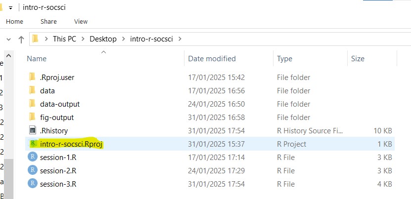
Double click on the file. Rstudio should launch with your project loaded!
Re-run the
library(tidyverse)andread_csvportion in the previous session (the code is also on the next slide if you missed last week’s session)
Optional (Though best practice):
- Make sure that
Environmentpanel is empty (click on broom icon to clean it up). - Clear the
ConsoleandPlotstoo.
Refresher: Loading from CSV into a dataframe
Use read_csv from readr package (part of tidyverse) to load our World Values Survey data. More information about the data can be found under the Dataset tab in the course website.
Why do we need to clean our data?
- Researchers spend 60-80% of their time on data preparation - investing in proper wrangling upfront saves hours of debugging and rework later.
- Poor data quality costs projects or organizations millions annually(!), and even one misclassified data point can skew entire analyses.
- Clean data improves the workflow for statistical tests and can reveal hidden patterns that aren’t visible in messy datasets
- Well-documented data cleaning makes research transparent and reproducible, benefiting both future-you and collaborators.
Why do it in R? Can’t I do this on excel?
- R code creates a permanent record of exactly what you did - Excel clicks and manual edits are hard to track and reproduce (unless you note down what you did).
- R handles dates, times, text, and mixed data types much more reliably than Excel.
- Excel can automatically “correct” your data in unwanted ways (like converting your dates from DDMMYY to MMDDYY)
- Write the cleaning code once, apply it to multiple datasets or when data updates. Whereas Excel requires manual repetition of the same steps each time.
- Complex joins, reshaping, and conditional operations that would take many Excel steps can be done in a few lines of R code.
- R scripts can be easily shared, version controlled, and integrated into reproducible workflows
What do I need to know before we begin?
- Always examine your data first (
glimpse(),summary(),str()) before cleaning. - Never overwrite your raw data files
- Budget extra time for data cleaning - it almost always takes longer than expected!
- Having a clear understanding of the desired data shape is essential as real data often differs from what you imagine! Refer to codebook, actual questionnaire, appendix for guidance.
- Look out for outliers!
- Remember: Data cleaning techniques differ based on the problems, data type, and the research questions you are trying to answer. Various methods are available, each with its own trade-offs.
The tools we’re going to use: dplyr and tidyr from tidyverse
Packages from
tidyverse. (click here to go to the tidyverse homepage)Posit have created cheatsheets here! (you can have this open in another tab for reference for this session!)
dplyr cheatsheet | pdf version (I personally prefer this PDF version since it’s more visual)
Most of the time, these are the ones that you will use quite often:
drop_na()- remove rows with null valuesselect()- to select column(s) from a dataframefilter()- to filter rows based on criteriamutate()- to compute new columns or edit existing onesif_else()andcase_when()- to be used with mutate when we want to compute/edit columns based on multiple criteriagroup_by()andsummarize()- group data and summarize each group
More advanced ones which is not covered in the workshop (see appendix for examples)
Joining multiple dataframes’ columns:
left_join(),right_join(),inner_join(),full_join()Joining multiple dataframes’ rows:
bind_rows()Splitting or combining cells:
unite(),separate_wider_delim(),separate_long_delim()
Additionally: you may need the forcats cheatsheet here: https://raw.githubusercontent.com/rstudio/cheatsheets/main/factors.pdf
forcats is also part of tidyverse, specifically used to handle factor data.
Why are we using tidyverse? Is it a must?
It’s not a must, but it’ll be make our job much easier! Key advantages:
- More ‘English’ looking code and thus more intuitive for beginners
- Tidyverse follow consistent syntax patterns - first argument is always the data to work on, followed by the function name i.e the things that we want to do on to the data.
- Tidyverse gives clearer, more helpful error messages
Example:
Scenario: Data wrangling activities with WVS data
Scenario: We are research assistants analyzing patterns in values, wellbeing, and demographics across four Asian countries: Hong Kong SAR, Indonesia, Malaysia, and Turkey.
Our team has been assigned to prepare and explore this dataset to understand how key factors (education, income level, urban/rural context, and emancipative/secular values) relate to life satisfaction and personal freedom across different generations.
To ensure analysis quality, we were instructed to discard incomplete data and prepare the dataset for statistical analyses in later sessions.
We can break down the steps as such:
Remove all rows with missing values (NA)
Check for duplicates
Select only the relevant columns.
- Though in our example, the columns in the sample dataset is ‘relevant’, i.e. will be used. To recap, the columns are
respondent_id, demographic columns (age,country,sex,urban_rural,income_level,marital_status,education), and the attitudinal columns (life_satisfaction,freedom_of_choice,financial_satisfaction,trust_people,importance_of_god,emancipative_values,secular_values)
- Though in our example, the columns in the sample dataset is ‘relevant’, i.e. will be used. To recap, the columns are
Filter for respondents aged 18 or older. Optionally, we can then arrange the dataset by age (oldest to youngest)
Create a new column
avg_satisfactionthat averageslife_satisfactionandfinancial_satisfactionas a combined well-being indicatorCreate age groups for each generation: “18-28”, “29-44”, “45-60”, “61+”
Once we did all of the wrangling above, we can save this “wrangled” version into another CSV as a “checkpoint”.
Let’s wrangle our data!
Step #1
A strategy I’d like to recommend: briefly read over the
dplyr+tidyrdocumentation, either the PDF or HTML version, and have them open on a separate tab so that you can refer to it quickly.
Remove all rows with empty values (NA) with drop_na()
The number of observations after removing NAs:
Interlude: Pipe Operator ( |> )
The pipe operator (|>) allows us to chain multiple operations without creating intermediate / temporary dataframes.
Super handy when we perform several data wrangling tasks using tidyverse in sequence.
Helps with readability, especially for complex operations.
Keyboard shortcut:
Ctrl+Shift+Mon Windows,Cmd+Shift+Mon Mac
Notice that we have to create a “temp” dataframe called wvs_data_clean in this method.
Step #2
Check for duplicates with distinct()
(Our data has no duplicates, but this is still a good practice to do, especially if we were combining data from multipe sources)
Step #3:
Select only the relevant columns: respondent_id, demographic columns, and attitudinal columns.
We can achieve this with select()!
Preview of the filtered data:
Rows: 5,102
Columns: 15
$ respondent_id          <dbl> 344070882, 344072005, 344071354, 344070282, 344…
$ country                <chr> "Hong Kong SAR", "Hong Kong SAR", "Hong Kong SA…
$ sex                    <chr> "Male", "Female", "Female", "Male", "Male", "Fe…
$ age                    <dbl> 62, 29, 55, 62, 41, 69, 25, 28, 62, 66, 57, 69,…
$ urban_rural            <chr> "Urban", "Urban", "Urban", "Urban", "Urban", "U…
$ income_level           <chr> "Medium", "Low", "Medium", "Low", "Medium", "Me…
$ marital_status         <chr> "Married", "Single", "Separated", "Married", "S…
$ education              <chr> "Middle", "Middle", "Higher", "Lower", "Middle"…
$ life_satisfaction      <dbl> 8, 2, 7, 7, 7, 5, 4, 6, 10, 5, 8, 7, 5, 6, 5, 8…
$ freedom_of_choice      <dbl> 7, 3, 5, 8, 6, 6, 5, 6, 10, 5, 8, 6, 5, 5, 7, 1…
$ financial_satisfaction <dbl> 7, 2, 6, 9, 6, 5, 4, 5, 8, 5, 8, 7, 5, 5, 5, 8,…
$ trust_people           <chr> "Trusted", "Not trusted", "Trusted", "Not trust…
$ importance_of_god      <dbl> 1, 1, 6, 3, 6, 5, 3, 7, 9, 3, 8, 5, 1, 5, 3, 10…
$ emancipative_values    <dbl> 0.7133333, 0.8263889, 0.6137963, 0.4725926, 0.5…
$ secular_values         <dbl> 0.5250000, 0.6941667, 0.4838889, 0.6794444, 0.6…
Step #4:
Filter for respondents aged 18 or older. Optionally, we can then arrange the dataset by age (oldest to youngest)
Checking the structure:
# A tibble: 6 × 15
  respondent_id country      sex     age urban_rural income_level marital_status
          <dbl> <chr>        <chr> <dbl> <chr>       <chr>        <chr>
1     792070014 Turkey       Male     95 Urban       Medium       Single
2     344070043 Hong Kong S… Male     91 Urban       Low          Married
3     344070645 Hong Kong S… Male     89 Urban       Low          Widowed
4     344070124 Hong Kong S… Male     88 Urban       Medium       Widowed
5     344070040 Hong Kong S… Male     88 Urban       Low          Married
6     344070082 Hong Kong S… Male     88 Urban       Low          Married
# ℹ 8 more variables: education <chr>, life_satisfaction <dbl>,
#   freedom_of_choice <dbl>, financial_satisfaction <dbl>, trust_people <chr>,
#   importance_of_god <dbl>, emancipative_values <dbl>, secular_values <dbl>
Step #5
Create a new column avg_satisfaction that averages life_satisfaction and financial_satisfaction as a combined wellbeing indicator.
We can achieve this with mutate()! (mutate() is to change or add new columns.)
Preview of the new column alongside the original ones:
# A tibble: 5,102 × 3
  life_satisfaction financial_satisfaction avg_satisfaction
              <dbl>                  <dbl>            <dbl>
1                 8                      5              6.5
2                10                      2              6
3                 4                      5              4.5
4                 1                      1              1
5                 9                      8              8.5
# ℹ 5,097 more rows
Step #6
Create age groups for each generation: “18-28”, “29-44”, “45-60”, “61+”
Preview of age groups:
# A tibble: 5,102 × 2
    age age_group
  <dbl> <chr>
1    95 61+
2    91 61+
3    89 61+
4    88 61+
# ℹ 5,098 more rows
Checkpoint 1 - saving our hard work into a CSV file
We have done some cleaning! Let’s save this cleaned data into a separate CSV file called “wvs_cleaned_v1.csv”
Check the data output folder to make sure the CSV is created!
Simple descriptive analysis
Once we are done with the wrangling part, we can proceed with simple descriptive analysis!
Prep: Before we proceed further, convert the appropriate categorical variables (country, sex, marital_status, urban_rural, income_level, education, trust_people) to Factor
Analysis 1: Generate summary statistics of life_satisfaction grouped by country
Analysis 2: Create a new column called
satisfaction_groupthat indicate whether each respondent has higher or lower than averagelife_satisfactionAnalysis 3: Reshape the data to show average satisfaction scores by country and age group
Prep before analysis: convert to factors
Let’s use the wvs_cleaned dataframe for this task.
Identify which columns can be converted to categorial data (factor). Convert the appropriate categorical variables (country, sex, marital_status, urban_rural, income_level, education, trust_people) to Factor.
We can do this with mutate() and as_factor() from forcats, another sub-package within tidyverse.
wvs_cleaned <- read_csv("data-output/wvs_cleaned_v1.csv")
wvs_cleaned <- wvs_cleaned |>
    mutate(
        country = as_factor(country),
        sex = as_factor(sex),
        marital_status = as_factor(marital_status),
        urban_rural = as_factor(urban_rural),
        income_level = as_factor(income_level),
        education = as_factor(education),
        trust_people = as_factor(trust_people)
    )

# check conversion result
str(wvs_cleaned)
Rstudio may auto-suggest as.factor() from base R. You can use this as well, but as_factor() is preferred since we are using tidyverse approach.
Prep before analysis: convert to factors
tibble [5,102 × 17] (S3: tbl_df/tbl/data.frame)
 $ respondent_id         : num [1:5102] 7.92e+08 3.44e+08 3.44e+08 3.44e+08 3.44e+08 ...
 $ country               : Factor w/ 4 levels "Turkey","Hong Kong SAR",..: 1 2 2 2 2 2 2 2 2 2 ...
 $ sex                   : Factor w/ 2 levels "Male","Female": 1 1 1 1 1 1 1 2 1 1 ...
 $ age                   : num [1:5102] 95 91 89 88 88 88 87 86 86 86 ...
 $ urban_rural           : Factor w/ 2 levels "Urban","Rural": 1 1 1 1 1 1 1 1 1 1 ...
 $ income_level          : Factor w/ 3 levels "Medium","Low",..: 1 2 2 1 2 2 2 1 1 2 ...
 $ marital_status        : Factor w/ 6 levels "Single","Married",..: 1 2 3 3 2 2 2 3 4 2 ...
 $ education             : Factor w/ 3 levels "Lower","Middle",..: 1 1 1 1 1 1 2 1 1 1 ...
 $ life_satisfaction     : num [1:5102] 8 10 4 1 9 10 8 5 8 5 ...
 $ freedom_of_choice     : num [1:5102] 1 1 5 9 10 9 5 1 8 5 ...
 $ financial_satisfaction: num [1:5102] 5 2 5 1 8 10 6 6 6 3 ...
 $ trust_people          : Factor w/ 2 levels "Not trusted",..: 1 1 1 1 1 1 1 1 2 1 ...
 $ importance_of_god     : num [1:5102] 10 6 9 1 6 10 1 1 2 1 ...
 $ emancipative_values   : num [1:5102] 0.25 0.339 0.464 0.657 0.471 ...
 $ secular_values        : num [1:5102] 0.151 0.345 0.401 0.597 0.313 ...
 $ avg_satisfaction      : num [1:5102] 6.5 6 4.5 1 8.5 10 7 5.5 7 4 ...
 $ age_group             : chr [1:5102] "61+" "61+" "61+" "61+" ...
Prep before analysis: convert to factors (shortcut ver.)
If we have a lot of columns to convert, that might be troublesome to type! This is where across() can come in handy. across(column selection, function) is to apply the same function or a set of functions to multiple columns in a single mutate () or summarize () function.
Let’s first define a character vector that contains the names of columns we plan to convert.
We will use this vector with mutate() and across(). We tell tidyverse to convert all of the columns with the help of all_of()
across() is used for applying the same function to multiple columns in a single mutate() or summarise() operation.
Prep before analysis: convert to factors (shortcut ver.)
tibble [5,102 × 17] (S3: tbl_df/tbl/data.frame)
 $ respondent_id         : num [1:5102] 7.92e+08 3.44e+08 3.44e+08 3.44e+08 3.44e+08 ...
 $ country               : Factor w/ 4 levels "Turkey","Hong Kong SAR",..: 1 2 2 2 2 2 2 2 2 2 ...
 $ sex                   : Factor w/ 2 levels "Male","Female": 1 1 1 1 1 1 1 2 1 1 ...
 $ age                   : num [1:5102] 95 91 89 88 88 88 87 86 86 86 ...
 $ urban_rural           : Factor w/ 2 levels "Urban","Rural": 1 1 1 1 1 1 1 1 1 1 ...
 $ income_level          : Factor w/ 3 levels "Medium","Low",..: 1 2 2 1 2 2 2 1 1 2 ...
 $ marital_status        : Factor w/ 6 levels "Single","Married",..: 1 2 3 3 2 2 2 3 4 2 ...
 $ education             : Factor w/ 3 levels "Lower","Middle",..: 1 1 1 1 1 1 2 1 1 1 ...
 $ life_satisfaction     : num [1:5102] 8 10 4 1 9 10 8 5 8 5 ...
 $ freedom_of_choice     : num [1:5102] 1 1 5 9 10 9 5 1 8 5 ...
 $ financial_satisfaction: num [1:5102] 5 2 5 1 8 10 6 6 6 3 ...
 $ trust_people          : Factor w/ 2 levels "Not trusted",..: 1 1 1 1 1 1 1 1 2 1 ...
 $ importance_of_god     : num [1:5102] 10 6 9 1 6 10 1 1 2 1 ...
 $ emancipative_values   : num [1:5102] 0.25 0.339 0.464 0.657 0.471 ...
 $ secular_values        : num [1:5102] 0.151 0.345 0.401 0.597 0.313 ...
 $ avg_satisfaction      : num [1:5102] 6.5 6 4.5 1 8.5 10 7 5.5 7 4 ...
 $ age_group             : chr [1:5102] "61+" "61+" "61+" "61+" ...
Analysis 1 - summary stats of life_satisfaction for each country
Generate summary statistics such as count (n), mean, median, and standard deviation of life_satisfaction grouped by country.
We can achieve this with group_by() and summarise(). It will contain one column for each grouping variable and one column for each of the summary statistics that you have specified.
What if we want to save this into a CSV? What if we also want to group by country AND age_group?
Analysis 1 - summary stats of life_satisfaction for each country
# A tibble: 4 × 5
  country           n mean_satisfaction median_satisfaction sd_satisfaction
  <chr>         <int>             <dbl>               <dbl>           <dbl>
1 Indonesia      1301              7.63                   8            2.39
2 Malaysia       1313              6.99                   7            1.75
3 Hong Kong SAR  1272              6.61                   7            1.80
4 Turkey         1216              6.48                   7            1.85
Analysis 2 - How many has below and average life_satisfaction?
Create a new column called satisfaction_group that indicate whether each respondent has higher or lower than average life_satisfaction
Analysis 2 - How many has below and average life_satisfaction?
# A tibble: 5,102 × 18
   respondent_id country     sex     age urban_rural income_level marital_status
           <dbl> <chr>       <chr> <dbl> <chr>       <chr>        <chr>
 1     792070014 Turkey      Male     95 Urban       Medium       Single
 2     344070043 Hong Kong … Male     91 Urban       Low          Married
 3     344070645 Hong Kong … Male     89 Urban       Low          Widowed
 4     344070124 Hong Kong … Male     88 Urban       Medium       Widowed
 5     344070040 Hong Kong … Male     88 Urban       Low          Married
 6     344070082 Hong Kong … Male     88 Urban       Low          Married
 7     344070833 Hong Kong … Male     87 Urban       Low          Married
 8     344070437 Hong Kong … Fema…    86 Urban       Medium       Widowed
 9     344070274 Hong Kong … Male     86 Urban       Medium       Separated
10     344070159 Hong Kong … Male     86 Urban       Low          Married
# ℹ 5,092 more rows
# ℹ 11 more variables: education <chr>, life_satisfaction <dbl>,
#   freedom_of_choice <dbl>, financial_satisfaction <dbl>, trust_people <chr>,
#   importance_of_god <dbl>, emancipative_values <dbl>, secular_values <dbl>,
#   avg_satisfaction <dbl>, age_group <chr>, satisfaction_group <chr>
Analysis 3 - What’s the average satisfaction scores for each country and age group?
Show the average satisfaction scores by country and age group in wide data format
# A tibble: 4 × 5
# Groups:   country [4]
  country       `18-28` `29-44` `45-60` `61+`
  <chr>           <dbl>   <dbl>   <dbl> <dbl>
1 Hong Kong SAR    6.31    6.33    6.57  7.26
2 Indonesia        7.90    7.53    7.57  7.55
3 Malaysia         7.05    6.91    7.01  7.14
4 Turkey           6.57    6.54    6.36  6.2
Long vs Wide Data
Long data:
Each row is a unique observation –> for a single observational unit, there might be multiple rows.
There is a separate column indicating the variable or type of measurements.
This format is more “understandable” by R, more suitable for visualizations, especially those involving grouping, summarizing, or visualizing data over time or across different categories. (which we’ll explore more next week!)
Wide data:
Each row contains values from variables.
Each column is a value in a variable –> the more values you have, the “wider” is the data.
Quick comparisons of different variables for a single entity.
This format is more intuitive for humans!
Long vs Wide Data: Examples
Long data:
| country | age_group | count |
|---|---|---|
| Hong Kong SAR | 18-28 | 191 |
| Hong Kong SAR | 29-44 | 384 |
| Hong Kong SAR | 45-60 | 412 |
| Hong Kong SAR | 61+ | 285 |
| Indonesia | 18-28 | 308 |
| Indonesia | 29-44 | 529 |
| Indonesia | 45-60 | 360 |
| Indonesia | 61+ | 104 |
| Malaysia | 18-28 | 379 |
| Malaysia | 29-44 | 511 |
| Malaysia | 45-60 | 349 |
| Malaysia | 61+ | 74 |
| Turkey | 18-28 | 329 |
| Turkey | 29-44 | 427 |
| Turkey | 45-60 | 430 |
| Turkey | 61+ | 30 |
Wide data:
| country | 18-28 | 29-44 | 45-60 | 61+ |
|---|---|---|---|---|
| Hong Kong SAR | 191 | 384 | 412 | 285 |
| Indonesia | 308 | 529 | 360 | 104 |
| Malaysia | 379 | 511 | 349 | 74 |
| Turkey | 329 | 427 | 430 | 30 |
Bonus: Deleting columns from dataframe
Let’s say I have this column called wrong_column that I want to remove:
Remove the wrong column with subset -:
# A tibble: 5,102 × 1
  country
  <chr>
1 Turkey
2 Hong Kong SAR
3 Hong Kong SAR
# ℹ 5,099 more rows
Recap
Import and read data into RStudio: Load external data files (like CSV or Excel) into R using functions such as
read_csv()to make the data available for analysis.Data wrangling with dplyr and tidyr (part of the tidyverse package): Use tidyverse functions to tidy and reshape datasets and perform tasks like selecting, filtering, and summarizing data.
Remove all rows with missing values (NA) and check for duplicates: Delete rows containing missing data using
drop_na()and identify or remove duplicate rows with functions likedistinct().Select only the relevant columns: Use
select()to keep only the columns needed for the analysis, focusing on important variables.Filter data based on criterion and arrange data: Apply
filter()to keep rows meeting specific conditions and usearrange()to sort data by one or more columns.Convert categorical variables to Factor data: Use
mutate()andas_factor.Create new columns: Generate or modify columns using
mutate(), often by transforming or combining existing columns.
End of Session 2!
Next session: Descriptive statistics and data visualization with ggplot2 package - we’ll create visualizations to explore patterns in life satisfaction, values, and demographics across countries!
Quiz Time! (compulsory)
Scan the QR Code below to assess your understanding of data wrangling in R using the tidyverse package. All questions are required and each is worth 1 mark.

To try at home: Exercise 1
Now that we have a new file, load this new wvs_cleaned_v1.csv into a new dataframe called wvs_cleaned. Filter to respondents from Indonesia who live in Urban areas. Show only the respondent_id, country, urban_rural, and age. Use glimpse() or print() to check the result! (you can chain these functions at the end)
Step 1: Load the new file
Step 2: Do the filtering and selecting, and then show result
Show answer
Rows: 326
Columns: 4
$ respondent_id <dbl> 360070522, 360070490, 360072309, 360070795, 360071345, 3…
$ country       <chr> "Indonesia", "Indonesia", "Indonesia", "Indonesia", "Ind…
$ urban_rural   <chr> "Urban", "Urban", "Urban", "Urban", "Urban", "Urban", "U…
$ age           <dbl> 76, 74, 71, 70, 68, 68, 67, 66, 66, 65, 65, 65, 65, 64, …
To try at home: Exercise 2
Generate a summary stats of age grouped by country and sex. The summary stats should include mean, median, max, min, std, and n (number of observations). It should look something like this:
To try at home: Exercise 2
# A tibble: 8 × 8
# Groups:   country [4]
  country       sex    observation mean_age median_age oldest youngest std_dev
  <chr>         <chr>        <int>    <dbl>      <dbl>  <dbl>    <dbl>   <dbl>
1 Hong Kong SAR Female         687     46.8         46     86       18    15.2
2 Hong Kong SAR Male           585     47.3         47     91       18    16.9
3 Indonesia     Female         713     38.3         37     78       18    12.8
4 Indonesia     Male           588     41.4         41     80       18    13.9
5 Malaysia      Female         656     37.7         35     80       18    12.8
6 Malaysia      Male           657     39.0         36     79       18    13.6
7 Turkey        Female         615     40.1         38     80       18    12.5
8 Turkey        Male           601     38.2         36     95       18    12.8
Appendix
Advanced tidyr and dplyr features you may need in the future.
Joining DataFrames by column
Let’s assume we have two DataFrames customers and orders
customers dataframe:
(Notice that the ID is 1, 2, and 3)
  id  name
1  1 Alice
2  2   Bob
3  3 Carol
orders dataframe
(Notice that the ID is 1, 2, and 4)
  id amount
1  1    100
2  2    200
3  4    150
left_join() to keep all rows from the left table i.e. customers
right_join() to keep all rows from the right table i.e. orders
inner_join() to keep only matching rows
full_join() to keep all rows from both tables
bind_rows() to stack rows from two different dataframes
Let’s say we have the following dataframes
Stack them together:
Splitting and combining cells
Let’s say we have the following dataframe
  first  last         full_address
1  John   Doe 123 Main St, NYC, NY
2  Jane Smith  456 Oak Ave, LA, CA