Session 5: Regression and Presenting Your Result
Today’s Outline
Today extends Session 4’s map: now the type of your outcome picks your model.
- Linear regression — for continuous outcomes
- one continuous predictor
- multiple continuous predictor
- one categorical predictor
- Logistic regression — for binary (yes/no) outcomes
- one continuous predictor
- one categorical predictor
- Presenting & reporting your results
- (bonus) Quarto show-and-tell
Open your project
Go to the folder where you put your project for this workshop
Find a file with
.Rprojextension - this is the R project file that holds all the information about your project.
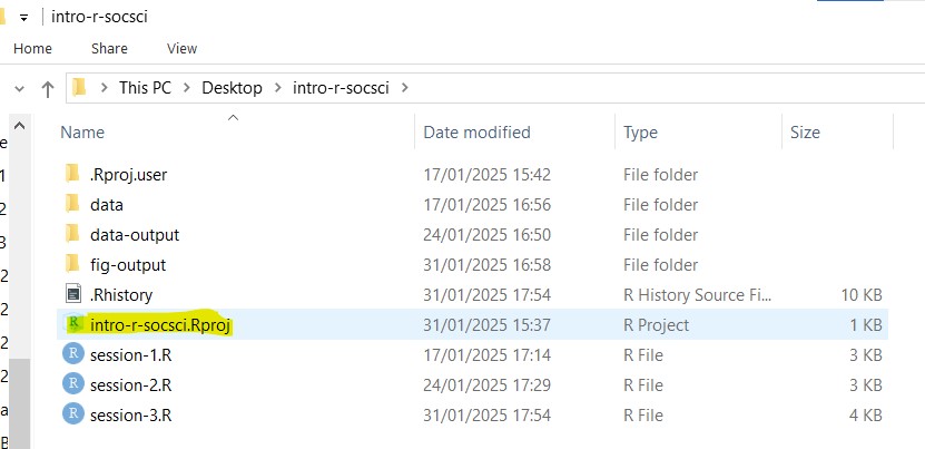
- Double click on the file. Rstudio should launch with your project loaded!
Set up for today
Today’s main flow runs on tidyverse + huxtable (for result tables). car and DescTools (from Session 1) are each used once via the car:: / DescTools:: prefix.
- Create a new R script called
session-5.R - Paste this in:
gtsummary and apaTables produce prettier tables but have heavier dependencies — they’re optional, with examples in the appendix. huxtable is lighter, and it’s all we need today.
Load our data for today!
# read the CSV with WVS data
wvs_cleaned <- read_csv("data-output/wvs_cleaned_v1.csv")

# Convert categorical variables to factors
columns_to_convert <- c("country", "sex", "marital_status", "urban_rural", "income_level", "education", "trust_people", "age_group")

wvs_cleaned <- wvs_cleaned |>
    mutate(across(all_of(columns_to_convert), as_factor))

# peek at the data, pay attention to the data types!
glimpse(wvs_cleaned)
From tests to models
Session 4 asked “which test?” from your variable types.
Regression asks the same kind of question, but kind of decided by outcome’s type:
| Your outcome (Y) | Model | R function |
|---|---|---|
| Continuous | Linear regression | lm() |
| Binary (yes/no) | Logistic regression | glm(..., family = binomial) |
Simple Linear Regression
Simple Linear Regression: what is it?
Linear regression is a statistical method used to model the relationship between a dependent variable (outcome) and one or more independent variables (predictors) by fitting a linear equation to the observed data. The math formula looks like this:
\[Y = \beta_0 + \beta_1X + \varepsilon\]
- \(Y\) - the dependent variable; must be continuous
- \(X\) - the independent variable (if there are more than one, there will be \(X_1\) , \(X_2\) , and so on. This can be ordinal, nominal, or continuous
- \(\beta_0\) - the y-intercept. Represents the expected value of the dependent variable \(Y\) when independent variable(s) \(X\) are set to zero.
- \(\beta_1\) - the slope / coefficient for independent variable
- \(\varepsilon\) - the error term. (In some examples you might see this omitted from the formula).
This is the \(y = mx + c\) line from secondary school! \(\beta_0\) is the intercept (\(c\)), \(\beta_1\) is the slope (\(m\)). Regression’s job is to find the best-fitting \(m\) and \(c\) from your data.
Examples:
- Does a person’s secular values affect their life satisfaction?
- Do a person’s secular values and financial satisfaction affect their life satisfaction?
Linear Regression: One continuous predictor
Research Question: Does a person’s level of secular values influence their life satisfaction?
- The outcome/DV (\(Y\)):
life_satisfaction - The predictor/IV (\(X\)):
secular_values
secular_values is Welzel’s secular-values index, ranging from 0 (very traditional/religious) to 1 (very secular). Keep this 0–1 scale in mind when interpreting the coefficient!
Call:
lm(formula = life_satisfaction ~ secular_values, data = wvs_cleaned)

Residuals:
    Min      1Q  Median      3Q     Max
-6.7641 -1.1920  0.2271  1.3497  4.0281

Coefficients:
               Estimate Std. Error t value Pr(>|t|)
(Intercept)     7.79792    0.06045     129   <2e-16 ***
secular_values -2.43734    0.15230     -16   <2e-16 ***
---
Signif. codes:  0 '***' 0.001 '**' 0.01 '*' 0.05 '.' 0.1 ' ' 1

Residual standard error: 1.967 on 5100 degrees of freedom
Multiple R-squared:  0.04782,   Adjusted R-squared:  0.04763
F-statistic: 256.1 on 1 and 5100 DF, p-value: < 2.2e-16Call: the formula
Residuals: overview on the distribution of residuals (expected value minus observed value) – we can plot this to check for homoscedasticity
Coefficients: shows the intercept, the regression coefficients for the predictor variables, and their statistical significance
Residual standard error: the average difference between observed and expected outcome by the model. Generally the lower, the better.
R-squared & Adjusted R-squared: indicates the proportion of variation in the outcome that can be explained by the model (i.e. goodness of fit).
F-statistics: indicates whether the model as a whole is statistically significant and whether it explains more variance than just the baseline (intercept-only) model.
Narrating the results
Here is one possible way to narrate your result:
A linear regression analysis was conducted to assess the influence of secular values on life satisfaction in Hong Kong SAR, Indonesia, Malaysia, and Turkey. Secular values were a statistically significant, negative predictor of life satisfaction (B = -2.44, SE = 0.15, p < 0.001).
Because
secular_valuesranges from 0 to 1, the raw coefficient describes the change across the entire scale. It is easier to interpret in smaller steps: for each 0.1 increase in secular values, life satisfaction decreases by about 0.24 units (−2.44 × 0.1) — that is, more secular respondents reported slightly lower life satisfaction.
The model was statistically significant (F(1, 5100) = 256.13, p < 0.001) but explained only about 4.8% of the variance in life satisfaction (R² = 0.048).
Linear Regression: Multiple continuous predictors
Research Question: Do a person’s financial satisfaction and secular values affect their life satisfaction?
- The outcome/DV (\(Y\)):
life_satisfaction - The predictors/IV (\(X\)):
financial_satisfactionandsecular_values
Linear Regression: Multiple continuous predictors
Call:
lm(formula = life_satisfaction ~ financial_satisfaction + secular_values,
    data = wvs_cleaned)

Residuals:
    Min      1Q  Median      3Q     Max
-8.5036 -0.8939  0.0305  0.8466  5.9702

Coefficients:
                       Estimate Std. Error t value Pr(>|t|)
(Intercept)             4.36997    0.08547   51.13   <2e-16 ***
financial_satisfaction  0.51588    0.01046   49.32   <2e-16 ***
secular_values         -1.81378    0.12596  -14.40   <2e-16 ***
---
Signif. codes:  0 '***' 0.001 '**' 0.01 '*' 0.05 '.' 0.1 ' ' 1

Residual standard error: 1.619 on 5099 degrees of freedom
Multiple R-squared:  0.3554,    Adjusted R-squared:  0.3551
F-statistic:  1405 on 2 and 5099 DF,  p-value: < 2.2e-16
Possible way to explain the result
A multiple regression analysis was conducted to examine how financial satisfaction and secular values predict life satisfaction. Financial satisfaction was a strong positive predictor (B = 0.52, SE = 0.01, p < 0.001): for each one-unit increase in financial satisfaction (on the 1–10 scale), life satisfaction increased by about 0.52 units. Secular values were a significant negative predictor (B = -1.81, SE = 0.13, p < 0.001); since this variable ranges 0–1, a 0.1 increase in secular values corresponds to about a 0.18-unit decrease in life satisfaction.
The model was statistically significant (F(2, 5099) = 1405.49, p < 0.001) and explained about 35.5% of the variance in life satisfaction (R² = 0.355).
Reporting result: A sample regression table
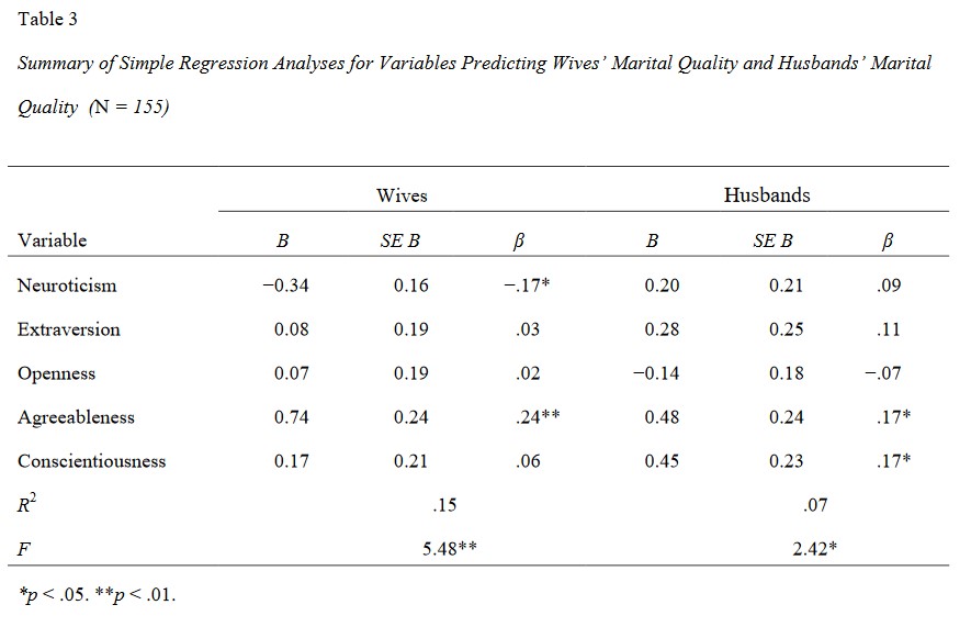
You might encounter different table formats when reporting regression results, but there are some key elements that should generally be included.
These are: the number of observations (\(N\)), the coefficients (B = unstandardized, raw coeff in original unit of measurements; \(\beta\) = standardized, converted to standard deviation units), standard errors (SE), confidence intervals (95% CI), and p-values. Other metrics to include are the \(R^2\) and \(F\) statistics.
Presenting your results with huxtable
huxreg() turns one or more models into a clean, copy-pasteable table — put several side by side to compare them:
For a single model, just huxreg(life_model1). The table appears in RStudio’s Viewer pane — select it, copy (Ctrl/Cmd + C), and paste into Word or Google Docs.
Presenting your results with huxtable
| model 1 | model 2 | |
|---|---|---|
| (Intercept) | 7.798 *** | 4.370 *** |
| (0.060) | (0.085) | |
| secular_values | -2.437 *** | -1.814 *** |
| (0.152) | (0.126) | |
| financial_satisfaction | 0.516 *** | |
| (0.010) | ||
| R squared | 0.048 | 0.355 |
| N | 5102 | 5102 |
| F | 256.128 | 1405.492 |
| P value | 0.000 | 0.000 |
| *** p < 0.001; ** p < 0.01; * p < 0.05. | ||
FYI: Multicollinearity
Caution! When doing regression-type of tests, watch out for multicollinearity.
Multicollinearity is a situation in which two or more predictor variables are highly correlated with each other. This makes it difficult to determine the specific contribution of each predictor variable to the relationship.
One way to check for it:
Assess the correlation between your predictor variables in your model using Variance Inflation Factor (VIF)
If they seem to be highly correlated (> 5 or so), one of the easiest (and somewhat acceptable) way is to simply remove the less significant predictor from your model :D
Linear Regression: One categorical predictor
Research Question: Explore the difference in life satisfaction between countries
- The outcome/DV (\(Y\)):
life_satisfaction - The predictor/IV (\(X\)):
country— an unordered categorical variable (the countries have no inherent order)
Note
Before proceeding with analysis, ensure that all the categorical variables involved are cast as factors! (We already did this in the load-data step.)
Continuing the analysis
The analysis summary should look like this:
Call:
lm(formula = life_satisfaction ~ country, data = wvs_cleaned)

Residuals:
    Min      1Q  Median      3Q     Max
-6.6311 -1.3544  0.3689  1.3876  3.5238

Coefficients:
                     Estimate Std. Error t value Pr(>|t|)
(Intercept)           6.47615    0.05637 114.887  < 2e-16 ***
countryHong Kong SAR  0.13627    0.07884   1.729    0.084 .
countryIndonesia      1.15490    0.07841  14.730  < 2e-16 ***
countryMalaysia       0.51319    0.07823   6.560 5.92e-11 ***
---
Signif. codes:  0 '***' 0.001 '**' 0.01 '*' 0.05 '.' 0.1 ' ' 1

Residual standard error: 1.966 on 5098 degrees of freedom
Multiple R-squared:  0.04935,   Adjusted R-squared:  0.04879
F-statistic: 88.22 on 3 and 5098 DF,  p-value: < 2.2e-16
When interpreting a categorical predictor in regression, one category is treated as the reference category, which serves as the baseline for comparison. In this case, the reference category corresponds to the intercept.
By default, the first category in the data is used as the reference — here that’s Turkey, so each coefficient is a country’s difference from Turkey.
Narrating the result
Here is one possible way to narrate your result:
A linear regression analysis was conducted to examine how country predicts life satisfaction, with Turkey as the reference group (intercept = 6.48, SE = 0.06). Compared to Turkey, respondents in Indonesia reported significantly higher life satisfaction (B = 1.15, SE = 0.08, p < 0.001), as did those in Malaysia (B = 0.51, SE = 0.08, p < 0.001). Hong Kong SAR scored slightly higher, but the difference was not statistically significant (B = 0.14, SE = 0.08, p = 0.084).
The model was statistically significant (F(3, 5098) = 88.22, p < 0.001) but explained only about 4.9% of the variance in life satisfaction (R² = 0.049).
Categorical predictor: changing the reference
Let’s change the reference category for country to “Malaysia” (our neighbour!).
Factor w/ 4 levels "Malaysia","Turkey",..: 2 3 3 3 3 3 3 3 3 3 ...Re-run the analysis with the new reference category
Categorical predictor: changing the reference
Call:
lm(formula = life_satisfaction ~ country, data = wvs_cleaned)

Residuals:
    Min      1Q  Median      3Q     Max
-6.6311 -1.3544  0.3689  1.3876  3.5238

Coefficients:
                     Estimate Std. Error t value Pr(>|t|)
(Intercept)           6.98934    0.05425 128.842  < 2e-16 ***
countryTurkey        -0.51319    0.07823  -6.560 5.92e-11 ***
countryHong Kong SAR -0.37692    0.07733  -4.874 1.13e-06 ***
countryIndonesia      0.64172    0.07689   8.345  < 2e-16 ***
---
Signif. codes:  0 '***' 0.001 '**' 0.01 '*' 0.05 '.' 0.1 ' ' 1

Residual standard error: 1.966 on 5098 degrees of freedom
Multiple R-squared:  0.04935,   Adjusted R-squared:  0.04879
F-statistic: 88.22 on 3 and 5098 DF,  p-value: < 2.2e-16
Changing baseline category for ordered factor
income_level is naturally ordered: Low < Medium < High. This is how we set (or change) that ordering explicitly as an ordered factor — put the levels in the sequence you want:
Ordered factors behave differently in regression
This slide is about reordering the levels of an ordered factor. But be careful: an ordered factor doesn’t have a “reference category” the way an unordered one does. In a regression, R codes it with polynomial contrasts (you’ll see coefficients labelled .L, .Q, .C — linear/quadratic/cubic trends), not “difference from a baseline group”. So if you want the “difference from a reference group” interpretation we’ve been using, keep the factor unordered and just relevel() it (as we did for country).
Let’s try this Linear Regression exercise! (5 mins)
Create a regression model called life_model4 that predicts the life_satisfaction score based on sex. The reference category should be ‘Male’
Code
Call:
lm(formula = life_satisfaction ~ sex, data = wvs_cleaned)

Residuals:
    Min      1Q  Median      3Q     Max
-6.0416 -1.0416  0.1785  1.1785  3.1785

Coefficients:
            Estimate Std. Error t value Pr(>|t|)
(Intercept)  6.82147    0.04082 167.110  < 2e-16 ***
sexFemale    0.22008    0.05642   3.901  9.7e-05 ***
---
Signif. codes:  0 '***' 0.001 '**' 0.01 '*' 0.05 '.' 0.1 ' ' 1

Residual standard error: 2.013 on 5100 degrees of freedom
Multiple R-squared:  0.002975,  Adjusted R-squared:  0.00278
F-statistic: 15.22 on 1 and 5100 DF,  p-value: 9.701e-05
Wait — how is this different from t-tests and ANOVA?
In case anyone’s been wondering the same thing! You don’t need this to run any analysis today — it’s just the “why” for the curious. Here’s the intuition:
- t-tests & ANOVA are framed around comparing group means — “are these groups different?”
- Correlation is framed around the strength & direction of a relationship — “do these two move together, and how tightly?” (symmetric — no outcome vs. predictor)
- Regression is framed around predicting an outcome from predictors — “what’s the relationship, and how big is it?”
They all belong to the general linear model family; they differ mainly in the types of variables they take and the question they’re framed around.
In a way, t-tests and ANOVA are special cases of linear regression
How they’re all equivalent to regression
| Traditional test | Equivalent regression | Gives the… |
|---|---|---|
| Two-group t-test | lm(y ~ binary_group) |
same p-value |
| One-way ANOVA | lm(y ~ multi_level_group) |
same F-statistic & p-value |
| Correlation | lm(y ~ continuous_x) |
same p-value |
A traditional ANOVA runs an omnibus test — “does any group differ?” — so you need a post-hoc test (Tukey’s, from Session 4) to find out which. Regression instead hands you specific coefficients: each one is a group’s difference from the reference category, directly. The underlying math is roughly the same!
So which one should I use?
- Short answer: it depends. Pick the framing that fits your question and what your reader expects (many fields/professors expect a “t-test” or “ANOVA” for a group comparison).
- Regression is the most general, flexible member of the family: many predictors, continuous + categorical mixed, and interactions.
- And logistic regression extends the very same idea to binary outcomes.
Binary Logistic Regression
Binary Logistic Regression - what is it?
Also known as simply logistic regression, it is used to model the relationship between a set of independent variables and a binary outcome.
These independent variables can be either categorical or continuous.
Binary Logistics Regression formula:
\[logit(P) = \beta_0 + \beta_1X_1 + \beta_2X_2 + … + \beta_nX_n\]
It can also be written like below, in which the \(logit(P)\) part is expanded:
\[P = \frac{1}{1 + e^{-(\beta_0 + \beta_1X)}}\]
The one-paragraph mental model
The outcome is now yes/no. You can’t fit a straight line to a 0/1, so we model the log-odds instead — the intimidating logit and \(e^x\) are just plumbing that keeps predicted probabilities between 0 and 1. What you actually read is the odds ratio: >1 = event more likely, <1 = less likely, for each 1-unit increase in X. If you hold onto just this, you’re set.
Binary Logistic Regression Examples
- Does a person’s age and education level influence whether they will vote Democrat or Republican in the US election?
- Does the number of hours spent studying impact a student’s likelihood of passing a module? (pass/fail outcome)
In essence, the goal of binary logistic regression is to estimate the probability of a specific event happening when there are only two possible outcomes (hence the term “binary”).
Binary Logistic Regression: One Continuous Predictor
Research Question: Does a participant’s sense of freedom of choice affect the likelihood of being satisfied with life?
The outcome/DV (\(Y\)):
satisfied- Our outcome is a continuous variable, but for the purpose of this workshop practice, let’s define the outcome as “Satisfied” if the life_satisfaction score is 7 or higher, and “not Satisfied” if the score is below 7.
The predictor/IV (\(X\)):
freedom_of_choice
We’re doing this only to have a binary dependent variable outcome to practice on. In real research, avoid chopping a continuous variable into two — it throws away information and statistical power. If your outcome is genuinely continuous, keep it continuous and use linear regression.
Dummy-coding dependent variable
Before we proceed with the calculations, we need to dummy code the dependent variable into 1 and 0, with 1 = Satisfied and 0 = Not Satisfied. More info on dummy coding here
# A tibble: 5,102 × 2
  life_satisfaction satisfied
              <dbl>     <dbl>
1                 8         1
2                10         1
3                 4         0
4                 1         0
5                 9         1
# ℹ 5,097 more rows
Conduct the analysis
Let’s conduct the analysis!
Call:
glm(formula = satisfied ~ freedom_of_choice, family = binomial,
    data = wvs_cleaned)

Coefficients:
                  Estimate Std. Error z value Pr(>|z|)
(Intercept)       -2.60780    0.12024  -21.69   <2e-16 ***
freedom_of_choice  0.45612    0.01714   26.62   <2e-16 ***
---
Signif. codes:  0 '***' 0.001 '**' 0.01 '*' 0.05 '.' 0.1 ' ' 1

(Dispersion parameter for binomial family taken to be 1)

    Null deviance: 6739.0  on 5101  degrees of freedom
Residual deviance: 5832.1  on 5100  degrees of freedom
AIC: 5836.1

Number of Fisher Scoring iterations: 3
Exponentiate the coefficients
If you recall the formula, the results are expressed in Logit Probability. As we typically report the result in terms of Odds Ratios (OR), perform exponentiation on the coefficients.
exp(coef(model)) is all you need to turn the log-odds into odds ratios, which is the numbers you report. (A formatted table version using tbl_regression() is in the appendix.)
Model significance (χ²) and R² for logistic
glm() doesn’t print a χ² or an R², so we ask DescTools::PseudoR2() for them. G2 is the model χ² (goodness-of-fit test vs. a no-predictor model); Nagelkerke is the pseudo-R² most commonly reported:
There are several pseudo-R² flavors (McFadden, Cox-Snell, …). Pick one and be consistent — Nagelkerke is a safe default. (The full list, and how to compute the χ² by hand, are in the appendix.)
Possible interpretation of the result
Possible interpretation:
(The intercept isn’t typically interpreted as an odds ratio, so we’ll ignore that for now)
A logistic regression was performed to ascertain the effects of freedom of choice on the likelihood that individuals will be satisfied with life versus not satisfied. The logistic regression model was statistically significant, χ²(1, N = 5102) = 906.91, p < .001.
The model explained about 22.2% (Nagelkerke R²) of the variance in life satisfaction. Freedom of choice was associated with an increased likelihood of being satisfied with life (OR = 1.58, 95% CI [1.53, 1.63], p < .001), indicating that for each one-unit increase in freedom of choice (1-10), the odds of being satisfied with life increased by about 58%.
Recap - why do I need to report these?
χ² (Chi-squared) goodness of fit tests whether your model fits the data significantly better than a null model (model with no predictors).
“Standard” R-squared isn’t typically reported for logistic regression because it’s not as meaningful as it is in linear regression. But we do still want to see how much of the variance in the data can be explained by the model.
Pseudo R-squared tries to mimic traditional R-squared by showing how much of the variation in the outcome your model explains, but it’s adjusted to work with binary outcomes. It’s sort of answering the question of “How well does my model explain the data?”
It is possible to have a significant χ² (meaning your model is statistically significant and better than nothing) but a low Pseudo R-squared (showing it still doesn’t explain much variation). This isn’t contradictory - it just means your model is better than random guessing but there’s still a lot of unexplained variation. (Pretty common in social sciences; after all, human behaviours are complex!)
FYI - IRL sample of reporting Logistic Regression
Below is a sample of how you may want to narrate your result. Note the resulting values mentioned in the paragraph below.
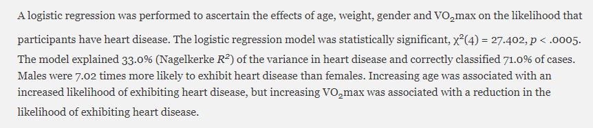
In a nutshell, you will most likely have to mention the p-value, the coefficients (for linear regressions), the Odds Ratios (for logistic regression) with the confidence intervals, the chi-squared (χ²), and the R-squared. You should also include these information in your regression table.
Binary Logistic Regression: One Categorical Predictor
Research Question: Does marital status affect the likelihood of being satisfied with life?
- The outcome/DV (\(Y\)):
satisfied - The predictor/IV (\(X\)):
marital_status- let’s set “Single” as the reference category!
Binary Logistic Regression: One Categorical Predictor
Call:
glm(formula = satisfied ~ marital_status, family = "binomial",
    data = wvs_cleaned)

Coefficients:
                                         Estimate Std. Error z value Pr(>|z|)
(Intercept)                               0.27975    0.05405   5.175 2.27e-07
marital_statusMarried                     0.38281    0.06546   5.848 4.97e-09
marital_statusWidowed                     0.16494    0.15749   1.047    0.295
marital_statusSeparated                  -0.27975    0.50291  -0.556    0.578
marital_statusDivorced                   -0.09743    0.16543  -0.589    0.556
marital_statusLiving together as married -0.21723    0.25590  -0.849    0.396

(Intercept)                              ***
marital_statusMarried                    ***
marital_statusWidowed
marital_statusSeparated
marital_statusDivorced
marital_statusLiving together as married
---
Signif. codes:  0 '***' 0.001 '**' 0.01 '*' 0.05 '.' 0.1 ' ' 1

(Dispersion parameter for binomial family taken to be 1)

    Null deviance: 6739.0  on 5101  degrees of freedom
Residual deviance: 6695.1  on 5096  degrees of freedom
AIC: 6707.1

Number of Fisher Scoring iterations: 4Get the χ² and R²
Same as before: G2 is the model χ² (goodness-of-fit), Nagelkerke is the pseudo-R² we’ll report.
Narrating the results
Possible interpretation:
(The intercept isn’t typically interpreted as an odds ratio, so we’ll ignore that for now)
A logistic regression was performed to ascertain the effects of marital status on the likelihood that individuals will be satisfied with life versus not satisfied. The logistic regression model was statistically significant, χ²(5, N = 5102) = 43.8, p < .001.
The model explained about 1.2% of the variance in life satisfaction (Nagelkerke R² ≈ 0.012 — read it off the
PseudoR2()output). Compared to single respondents (the reference group), married respondents had significantly higher odds of being satisfied with life (OR = 1.47, 95% CI [1.29, 1.67], p < .001) — roughly 47% higher odds. None of the other categories (widowed, divorced, separated, or living together) differed significantly from single respondents (all p > .05).
Presenting logistic results with huxtable
huxreg() works for glm() models too — here comparing both logistic models:
Heads-up: huxreg() shows the raw log-odds coefficients for a glm, not odds ratios — remember exp(coef(model)) for the ORs you report. It also omits pseudo-R², so note that separately from PseudoR2().
Presenting logistic results with huxtable
| freedom of choice | marital status | |
|---|---|---|
| (Intercept) | -2.608 *** | 0.280 *** |
| (0.120) | (0.054) | |
| freedom_of_choice | 0.456 *** | |
| (0.017) | ||
| marital_statusMarried | 0.383 *** | |
| (0.065) | ||
| marital_statusWidowed | 0.165 | |
| (0.157) | ||
| marital_statusSeparated | -0.280 | |
| (0.503) | ||
| marital_statusDivorced | -0.097 | |
| (0.165) | ||
| marital_statusLiving together as married | -0.217 | |
| (0.256) | ||
| N | 5102 | 5102 |
| logLik | -2916.042 | -3347.573 |
| AIC | 5836.084 | 6707.146 |
| *** p < 0.001; ** p < 0.01; * p < 0.05. | ||
Let’s try this Logistic Regression exercise! (5 mins)
Create a regression model called life_model7 that predicts the likelihood of being satisfied with life based on sex.
Bonus show-and-tell: Quarto
What are Markdown, R Markdown, and Quarto?
- Markdown — a lightweight, readable way to write formatted text (no messy HTML or LaTeX). Files end in
.md. - R Markdown — Markdown + live R code chunks, so text, code, and output (tables, plots) live in one document (
.Rmd). - Quarto — Posit’s next-generation, multi-language successor to R Markdown. It renders most
.Rmdfiles unchanged and can output HTML, Word, PDF, slides, and whole websites. - Fun fact: this entire course website and these slides are built in Quarto! (A quick R-Scripts-vs-Quarto comparison is in the appendix.)
How it all works

Illustration by Allison Horst (www.allisonhorst.com)
If you are interested to learn more about this…
SMU Libraries regularly host Quarto workshops every semester from week 2 to week 6, taught by Prof Kam Tin Seong.
Keep a lookout for these titles:
- R Ep.1: Making Your Research Reproducible with Quarto in RStudio
- R Ep.7: Creating Awesome Web Slides in Quarto with Revealjs
- R Ep.9: Building Website and Blog with Quarto
Best Practices + More Resources
R Best Practices
Use
<-for assigning values to objects.- Only use
=when passing values to a function parameter.
- Only use
Do not alter your raw data; save your wrangled/cleaned data into a new file and keep it separate from the raw data.
Make use of R projects to organize your data and make it easier to send over to your collaborators.
- Having said that, when it comes to coding project, the best way to collaborate is using GitHub or similar platforms.
Whenever possible and makes sense for your project, follow the common convention when naming your objects, scripts, and functions. One guide that you can follow is Hadley Wickham’s tidyverse style guide.
References for APA Guidelines on Reporting statistics
Do check with your professor on how closely you should follow the guidelines, or if there is any specific format required.
One last thing: you own the analysis
“Because the AI said so” is not an answer
Over five sessions you’ve learned to import, wrangle, visualize, and run real inferential tests in R. An AI assistant can now generate all of that code for you in seconds — and often it will do a decent job.
So what’s your job now? The parts the AI can’t be accountable for:
- Define the research questions and thus test for your variables — and being able to say why.
- Checking whether the result can be reasonably trusted — assumptions, sample size, plain common sense.
- Interpreting the output honestly.
- Disclosing the limitations plainly, even when they’re inconvenient.
When your professor, a reviewer, or a future employer asks “why did you run this analysis, and can I trust it?” — “Claude/ChatGPT told me to” is not a defensible answer. You are accountable for the work that carries your name.
Thank you for your participation 😄

All the best for your studies and academic journey! (manifesting excellent grades + internship for everyone who attended the workshop)
Need help with R or Quarto? Please don’t hesitate to contact us at bellar@smu.edu.sg or weixia@smu.edu.sg
Quiz Time! (compulsory)
Scan the QR Code below to assess your understanding of regression analysis and reporting results using R in social sciences. All questions are required and each is worth 1 mark.

Post-workshop survey
Please scan this QR code or click on the link below to fill in the post-workshop survey. It should not take more than 2-3 minutes.
Survey link: https://smusg.asia.qualtrics.com/jfe/form/SV_9Xhn2NY4vkA4GaO

Appendix
- Prettier tables with gtsummary & apaTables
- gtsummary summary tables
- Computing the logistic χ² by hand
- Other pseudo-R² methods
- R Scripts vs Quarto
We used huxtable in the main session. These gtsummary / apaTables alternatives produce nicer output but have heavier dependencies — the code here is shown for reference, not executed — run it live in RStudio (after install.packages() + library()) to see the tables.
Presenting regression tables: gtsummary (tbl_regression)
tbl_regression() makes clean, publication-style tables. For logistic models, exponentiate = TRUE reports odds ratios:
These render in RStudio’s Viewer pane — select the table, copy (Ctrl/Cmd + C), and paste into Word or Google Docs.
Table packages: apaTables
apaTables generates APA-formatted tables for correlation, ANOVA, and regression. Limited customisation. The online docs are for the development version (not what install.packages() gives you), so lean on the vignette. Documentation here
Example: a correlation table for life_satisfaction, financial_satisfaction, and freedom_of_choice
This creates a Word document with the table already formatted in APA style.
Table packages: gtsummary summary tables
Besides tbl_regression(), gtsummary can build descriptive / mean-difference tables with tbl_summary(). Documentation here
Example: mean-differences table grouped by sex
Computing the logistic χ² by hand
We used PseudoR2(..., which = "G2") to get the model χ². If you ever need it manually, it’s the drop in deviance from the null model:
- χ² = Null deviance − Residual deviance (both from the
summary()output) - df = Null df − Residual df (= number of predictors)
Other pseudo-R² methods
If you specifically need a different pseudo-R² (e.g. McFadden, Cox-Snell), PseudoR2() can return them all at once:
       McFadden     McFaddenAdj        CoxSnell      Nagelkerke   AldrichNelson
      0.1345762       0.1339826       0.1628528       0.2221449       0.1509272
VeallZimmermann           Efron McKelveyZavoina            Tjur             AIC
      0.2651922       0.1844291       0.2233348       0.1772867    5836.0841311
            BIC          logLik         logLik0              G2
   5849.1589069   -2916.0420655   -3369.4958907     906.9076503
R Scripts vs Quarto
R Scripts
Great for quick debugging, experiment
Preferred format if you are archiving your code to GitHub or data repository
More suitable for “production” tasks e.g. automating your data cleaning and processing, custom functions, etc.
Quarto
Great for report and presentation to showcase your research insights/process as it integrates code, narrative text, visualizations, and results.
Very handy when you need your report in multiple format, e.g. in Word and PPT.
Fun fact: the course website and slides are all made in Quarto